Control synthesis

Overview

LPVcore contains state-of-the-art analysis and controller synthesis algorithms for several model structures. On this page, a brief overview is given of the functionality available to perform analysis and controller synthesis. Firstly, an overview of the available analysis methods is provided. Secondly, the available algorithms for controller synthesis are presented. Finally, a short description of the algorithms that are used to solve the analysis and controller synthesis problems is given.

Analysis

General information

Suggested example

• synthesis/example_lpvnorm.m

Through the lpvnorm function, several methods are available to analyze the performance (and stability) of LPV systems. The supported LPV representations are LPVcore.lpvss and LPVcore.lpvidss objects with an affine scheduling-dependency, i.e., of the form

$$\begin{aligned} \xi x &= A(p) x + B(p) u, \\[4pt] y &= C(p) x + D(p)u , \end{aligned}$$

where $x$ is the state of the model, $u$ its input, and $y$ its output, $\xi=\frac{d}{dt}$ in continuous-time and $\xi=q^{-1}$ in discrete-time. Moreover, $A$, $B$, $C$, and $D$ are matrix functions of the form $M(p) = M_0 + \sum_{i=1}^{n_\mathrm{p}}M_i \, p_i$. Furthermore, grid-based LPV representations as LPVcore.lpvgridss objects are also supported by lpvnorm.

In the following table, an overview of the available performance metrics that can be analyzed is given. The corresponding type option for the lpvnorm command for each performance metric is also indicated. By default, if type is not specified, l2 is used.

Performance metric	IO relation*	Command
Induced $L_2$-gain	$\Vert y \Vert_2\leq\gamma\Vert u\Vert_2$	lpvnorm(sys,'l2')
Induced $L_\infty$-gain	$\Vert y \Vert_\infty\leq\gamma\Vert u\Vert_\infty$	lpvnorm(sys,'linf')
Generalized $H_2$ norm	$\Vert y \Vert_\infty\leq\gamma\Vert u\Vert_2$	lpvnorm(sys,'h2')
Passivity	$\int_0^T y(t)^\top u(t)\,dt\geq 0$	lpvnorm(sys,'passive')

*'$\Vert\cdot\Vert$' denotes the signal norm, see Definition 2.8 in [1] for more details.

The following code snippet shows how the induced $L_2$-gain of an LPV model can be computed:

p = preal('p', 'ct', 'Range', [0, 9]);

A = [0 1; - 1 - p, -3];
B = [0;1];
C = [1 0];
D = 0;
model = LPVcore.lpvss(A, B, C, D);

gam = lpvnorm(model, 'l2');

See synthesis/example_lpvnorm.m for more detailed examples.

Analysis options

Several options are available for lpvnorm. Namely, the following name-value pairs are available:

• SolverOptions: A structure containing the YALMIP solver settings. See also help sdpsettings. Default value: sdpsettings('verbose',0,'solver','sdpt3').
• NumericalAccuracy: An option to set the numerical accuracy parameter. A positive number that is used to ensure that the solved LMIs are negative or positive definite by enforcing that $\mathrm{LMI} \preceq -\alpha I$ or $\mathrm{LMI} \succeq \alpha I$, respectively, where $\alpha$ is the value of the numerical accuracy parameter. Default value: 1e-10.
• LinfOptions: A structure containing the options for $L_\infty$ based analysis. It needs to be constructed by using the linfOptions command. See below for more details. Default value: linfOptions().
• ParameterVaryingStorage: An option to indicate whether a parameter-varying storage function is considered (if at least one of the scheduling-variables has finite rate-bounds). Use 0 to indicate using a parameter-independent storage function, 1 to indicate parameter-dependency on all parameters with finite rate-bounds. For LPVcore.lpvgridss models, the user must specify a 'template storage function' in order to use a parameter-varying storage function. This template storage function is used in order to specify the parameter dependency of the used parameter-varying storage function. For example:

  >> p = preal('p', 'ct', 'RateBound', [-1 1]');
  >> stor = 1 + p + p^2;
  >> lpvnorm(sys, 'l2', 'ParameterVaryingStorage', stor)
  All the used parameters of the template storage function should have their rate bounds specified and their names should match the parameter names of the considered LPVcore.lpvgridss model. In continuous-time, the template storage function can only have a polynomial dependency, i.e., custom basis function through pbcustom cannot be used. Default value: 1 (for LPVcore.lpvss models), 0 (for LPVcore.lpvgridss models).
• Verbose: Option to turn progress messages on, 1, or off, 0. Default value: 1.

The options can be used by adding them as input arguments to the lpvnorm command, for example:

gam = lpvnorm(model, 'l2', 'Verbose', 0, 'NumericalAccuaracy', 1e-8);

or

gam = lpvnorm(model, 'l2', Verbose = 0, NumericalAccuaracy = 1e-8);

Controller synthesis

Output Feedback Synthesis

General information

Suggested example

• synthesis/example_lpvsyn.m

The lpvsyn command allows the user to synthesize various optimal (output-feedback) LPV state-space controllers $K$ for a given state-space LPV (generalized) plant $P$. Like for analysis, the lpvsyn command supports LPVcore.lpvss and LPVcore.lpvidss objects with an affine scheduling dependency, as well as LPVcore.lpvgridss objects.

It is assumed that the plant $P$ is of the form

$$\begin{aligned} \xi x &= A(p) x + B_\mathrm{w}(p)w + B_\mathrm{u}(p) u, \\[4pt] z &= C_\mathrm{z}(p)x + D_\mathrm{zw}(p)w + D_\mathrm{zu}(p) u,\\[4pt] y &= C_\mathrm{y}(p) x +D_\mathrm{yw}(p)w . \end{aligned}$$

where $x$ is the state of the model, $u$ its control input, $y$ its measured output, $w$ is the (generalized) disturbance channel, and $z$ is the (generalized) performance channel.

info

For controller synthesis for affine LPVcore.lpvss and LPVcore.lpvidss objects, it is assumed that $B_\mathrm{u},$ $C_\mathrm{y},$ $D_\mathrm{zu},$ and $D_\mathrm{yw}$ are constant matrices.

The synthesized controller $K$ resulting from running lpvsyn is of the form

$$\begin{aligned} \xi x_\mathrm{k} &= A_\mathrm{k}(p) x_\mathrm{k} + B_\mathrm{k}(p) u_\mathrm{k}, \\[4pt] y_\mathrm{k} &= C_\mathrm{k}(p) x_\mathrm{k} +D_\mathrm{k}(p)u_\mathrm{k} , \end{aligned}$$

which is connected to $P$ as in the following figure:

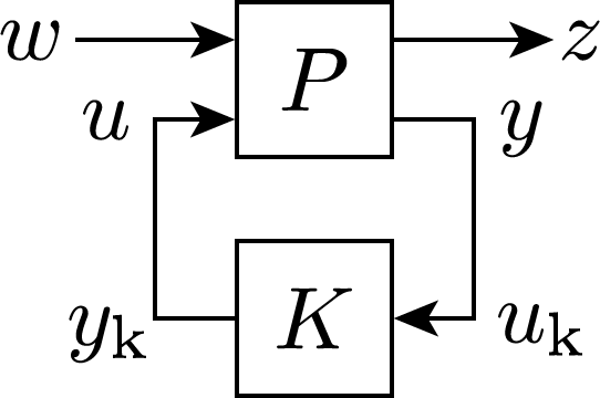
By default, for the closed-loop of $P$ and $K$, the $L_2$-gain from $w$ to $z$ is minimized to synthesize $K$. The considered performance metric can be adjusted by changing the Performance option through lpvsynOptions or by using one of the performance-specific synthesis functions, i.e., lpvl2syn, lpvlinfsyn, lpvh2syn, or lpvpassyn. The available performance metrics are given in the table below.

Performance metric	IO relation*	Command
Induced $L_2$-gain	$\Vert y \Vert_2\leq\gamma\Vert u\Vert_2$	Setting lpvsynOptions('Performance,'l2') for lpvsyn or using lpvl2syn
Induced $L_\infty$-gain	$\Vert y \Vert_\infty\leq\gamma\Vert u\Vert_\infty$	Setting lpvsynOptions('Performance,'linf') for lpvsyn or using lpvlinfsyn
Generalized $H_2$ norm	$\Vert y \Vert_\infty\leq\gamma\Vert u\Vert_2$	Setting lpvsynOptions('Performance,'h2') for lpvsyn or using lpvh2syn
Passivity	$\int_0^T y(t)^\top u(t)\,dt\geq 0$	Setting lpvsynOptions('Performance,'passive') for lpvsyn or using lpvpasssyn

The following code snippet shows how an $L_2$-gain optimal LPV controller can be synthesized for a plant $P$:

p = preal('p', 'ct', 'Range', [0, 9]);

A = [0 1; - 1 - p, -3];
B = [0 0;0 1];
C = [-1 0;-1 0];
D = [1 0;1 0];
P = LPVcore.lpvss(A, B, C, D);

ny = 1;
nu = 1;

[K, gam] = lpvsyn(P, ny, nu);

See synthesis/example_lpvsyn.m for more detailed examples.

Synthesis options

Various options related to controller synthesis can be set using the lpvsynOptions function. The following options, specified as name-value pairs, are available:

• Backoff: The factor which is used to back off from the optimal gain $\gamma$ that is found (to $\alpha\cdot\gamma$, where $\alpha$ is the Backoff value) in order to reduce numerical errors, since the true optimal solution is often close to singular. Default value: 1.01.
• Dependency: A logical array (1x4 or 4x1) which indicates which controller matrices, corresponding to $A$, $B$, $C$ and $D$-matrix, should have parameter-dependency. In case of the transformation method, these apply to the transformed controller matrices, i.e., $\mathcal{A}_\mathrm{k}$, $\mathcal{B}_\mathrm{k}$, $\mathcal{C}_\mathrm{k}$, and $\mathcal{D}_\mathrm{k}$ in Section 2.5.3. in [1] or similarly $K$, $L$, $M$, and $N$ in Section 4.2.2. in [5]. Default value: [1 1 1 1].
• DirectFeedthrough: An option to indicate if the synthesized controller should have direct feedthrough 1 or not 0, i.e., if the controller has a $D_\mathrm{k}$-matrix or not. Default value: 1.
• ImproveConditioning: An option to indicate if extra optimization problems are solved to improve the conditioning of the found solutions. Default value: 1.
• LinfOptions: An option to set the options for $L_\infty$-based controller synthesis. Needs to be constructed by using the linfOptions command. See below for more details. Default value: linfOptions().
• Method: An option to indicate what method to use internally to solve the controller synthesis problem. Possible values are transformation and projection. Using transformation, a nonlinear transformation is applied to the unknown variables (such as the controller matrices) in order to construct the LMIs for controller synthesis. The optimization problem is solved in these new variables, which are then used to compute the controller state-space matrices $A_\mathrm{k}$, $B_\mathrm{k}$, $C_\mathrm{k}$, and $D_\mathrm{k}$ through the nonlinear transformation. Using projection, the controller state-space matrices are 'projected' away from the LMIs. Then, the optimization problem is solved for these LMIs which do not contain the controller state-space matrices. Then, an extra LMI is solved, corresponding to the closed-loop system containing the controller state-space matrices as unknowns, in order to obtain the controller state-space matrices. The transformation method often gives better numerical results. However, for continuous-time systems, only the projection method allows for controller synthesis with a parameter-varying storage function. Default value: transformation. NumericalAccuracy: An option to set the numerical accuracy parameter. A positive number that is used to ensure that the solved LMIs are negative or positive definite by enforcing that $\mathrm{LMI} \preceq -\alpha I$ or $\mathrm{LMI} \succeq \alpha I$, respectively, where $\alpha$ is the value of the numerical accuracy parameter. Default value: 1e-8.
• ParameterVaryingStorage: An option to indicate whether a parameter-varying storage function is considered (if at least one of the scheduling-variables has finite rate-bounds). Use 0 to indicate using a parameter-independent storage function, 1 to indicate parameter-dependency on all parameters with finite rate-bounds, or set to [] to let lpvsyn decide if an parameter-varying storage function can be used or not. Similar as for lpvnorm, for LPVcore.lpvgridss models the user must specify a 'template storage function' in order to use a parameter-varying storage function. This template storage function is used in order to specify the parameter dependency of the used parameter-varying storage function. For example:

  >> p = preal('p', 'ct', 'RateBound', [-1 1]');
  >> stor = 1 + p + p^2;
  >> lpvnorm(sys, 'l2', 'ParameterVaryingStorage', stor)
  All the used parameters of the template storage function should have their rate bounds specified and their names should match the parameter names of the considered LPVcore.lpvgridss model. In continuous-time, the template storage function can only have a polynomial dependency, i.e., custom basis function through pbcustom cannot be used. Default value: [] (for LPVcore.lpvss models), 0 (for LPVcore.lpvgridss models).
• ParameterVaryingStorageOption: This options allows the user to choose between two different parameter-varying storage parameterizations. More specifically, this allows the user to either synthesize a controller corresponding third (by setting this option to 1) or fourth row (by setting this option to 2) in Table I in [3]. Neither option is in general better and which option will achieve better performance will depend on the specific control problem (and plant) that is considered. This option is currently only available for continuous-time controller synthesis problems. Default value: 1.
• Performance: An option to set the performance metric that is considered for controller synthesis. Possible values are: 'linf', 'l2', 'h2', and 'passive'. Default value: 'l2'.
• PoleConstraint: An option to set constraints on the closed-loop eigenvalues for controller synthesis. It needs to be constructed using the poleConstraintOptions command. See below for more details. Default value: poleConstraintOptions().
• SolverOptions: A structure containing the YALMIP solver settings. See also help sdpsettings. Default value: sdpsettings('verbose', 0, 'solver', 'sdpt3').
• Verbose: An option to turn progress messages on, 1, or off, 0. Default value: 1.

Usage example:

synOptions = lpvsynOptions('Backoff', 1.1, 'Performance', 'linf');

or

synOptions = lpvsynOptions(Backoff = 1.1, Performance = 'linf');

The synOptions variable can then be used with lpvsyn as follows:

K = lpvsyn(sys, ny, nu, synOptions);

State-feedback synthesis

General information

Suggested example

• synthesis/example_lpvsynsf.m

The lpvsynsf command allows the user to synthesize state-feedback LPV controllers $K$ for a state-space LPV (generalized) plant $P$. Similar to output-feedback controller synthesis using lpvsyn, the lpvsynsf command supports LPVcore.lpvss and LPVcore.lpvidss objects with an affine scheduling dependency, as well as LPVcore.lpvgridss objects.

For state-feedback synthesis, it is assumed that the plant $P$ is of the form

$$\begin{aligned} \xi x &= A(p) x + B_\mathrm{w}(p)w + B_\mathrm{u}(p) u, \\[4pt] z &= C_\mathrm{z}(p)x + D_\mathrm{zw}(p)w + D_\mathrm{zu}(p) u,\\[4pt] \end{aligned}$$

where again $x$ is the state of the model, $u$ its control input, $w$ is the (generalized) disturbance channel, and $z$ is the (generalized) performance channel.

The synthesized controller $K$ resulting from running lpvsynsf is of the form

$$u = K(p)x$$

and is given as a parameter-varying matrix object $K$.

By default, the $L_2$-gain from $w$ to $z$ is minimized to synthesize $K$. Similarly, as for lpvsyn, the considered performance metric can be adjusted by changing the Performance option through lpvsynsfOptions or by using one of the performance-specific synthesis functions, i.e., lpvl2synsf, lpvlinfsynsf, lpvh2synsf, or lpvpassynsf. The available performance metrics are given in the table below.

Performance metric	IO relation*	Command
Induced $L_2$-gain	$\Vert y \Vert_2\leq\gamma\Vert u\Vert_2$	Setting lpvsynsfOptions('Performance,'l2') for lpvsynsf or using lpvl2synsf
Induced $L_\infty$-gain	$\Vert y \Vert_\infty\leq\gamma\Vert u\Vert_\infty$	Setting lpvsynsfOptions('Performance,'linf') for lpvsynsf or using lpvlinfsynsf
Generalized $H_2$ norm	$\Vert y \Vert_\infty\leq\gamma\Vert u\Vert_2$	Setting lpvsynsfOptions('Performance,'h2') for lpvsynsf or using lpvh2synsf
Passivity	$\int_0^T y(t)^\top u(t)\,dt\geq 0$	Setting lpvsynsfOptions('Performance,'passive') for lpvsynsf or using lpvpasssynsf

The following code snippet shows how an $L_2$-gain optimal state-feedback LPV controller can be synthesized for a plant $P$:

p = preal('p', 'ct', 'Range', [0, 9]);

A = [0 1; - 1 - p, -3];
B = [0 0;0 1];
C = [-1 0];
D = [1 0];
P = LPVcore.lpvss(A, B, C, D);

nu = 1;

[K, gam] = lpvsynsf(P, nu);

See synthesis/example_lpvsynsf.m for more detailed examples.

Synthesis options

Various options related to state-feedback controller synthesis can be set using the lpvsynsfOptions function. The majority of the options specified by lpvsynsfOptions are the same as the ones in lpvsynOptions, see above. Next, we will list all options that are available, and we will give a description for the options that differ from the ones of lpvsynOptions.

• Backoff
• Dependency: A logical value which indicates if the state-feedback matrix $K$ should be parameter-dependent, 1, or not, 0. Default value: 1.
• ImproveConditioning
• LinfOptions
• NumericalAccuracy
• ParameterVaryingStorage
• ParameterVaryingStorageOption
• Performance
• PoleConstraint
• SolverOptions
• Verbose

Usage example:

synOptions = lpvsynsfOptions('Backoff', 1.1, 'Performance', 'linf');

or

synOptions = lpvsynsfOptions(Backoff = 1.1, Performance = 'linf');

The synOptions variable can then be used with lpvsynsf as follows:

K = lpvsynsf(sys, nu, synOptions);

General Options

$L_\infty$-based analysis and controller synthesis options

Analysis and controller synthesis for $L_\infty$ performance work by carrying out a line-search over a slack variable $\lambda$ in order to compute the minimal $L_\infty$-gain that the system satisfies. The line-search works by first optimizing $\gamma$ (which corresponds to the $L_\infty$-gain) for a fixed number of values for $\lambda$. Afterwards, a bisection-based search algorithm (based on the Golden-ratio) is used between the interval of $\lambda$'s that attain the lowest $\gamma$'s in order to optimize the value of $\gamma$ further. In order to adjust the settings related to this procedure, the user can use the linfOptions command. The command allows the user to adjust the following settings by specifying name-value pairs:

• AccuracyLambda: Allows specifying the maximum $\lambda$ search interval during the bisection-based search. If the $\lambda$ interval is smaller than this value, the search is completed. Default value: 1e-3.
• LambdaGrid: Array of values for $\lambda$ used for initial line-search. Default value: linspace(1e-8, 5, 15).
• MaxIterations: Maximum number of iterations for the bisection-based search phase. Default value: 25.

Usage example:

linfOpt = linfOptions('AccuracyLambda', 1e-4, 'MaxIterations', 30);

or

linfOpt = linfOptions(AccuracyLambda = 1e-4, MaxIterations = 30);

Pole constraint options

info

Support for pole constraints is currently only supported for continuous-time controller synthesis.

For controller synthesis, the closed-loop eigenvalues for frozen values of the scheduling-variable can be restricted to lie in a certain region in the complex plane. These constraints can be specified through the poleConstraintOptions command. Several regions can be specified as name-value pairs through the command. The options that are available are given in the table below. Specifying multiple constraint regions results in the intersection of these regions being taken as a constraint.

Name	Description	Inequality	Figure
Circle	Constraint eigenvalues to an open circle with radius 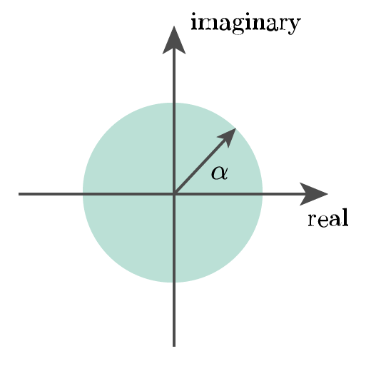$\alpha$	$\vert z \vert<\alpha$ with $\alpha>0$
LeftHalfPlane	Constraint eigenvalues to lie in the open left half-plane	$\mathrm{Re}(z) < \alpha$ with $\alpha\in\mathbb{R}$
RightHalfPlane	Constraint eigenvalues to lie in the open right half-plane	$\mathrm{Re}(z) > \alpha$ with $\alpha\in\mathbb{R}$
Sector	Constraint eigenvalues to a sector in the left half-plane with an angle of $\alpha$ [rad]	$\mathrm{Re}(z)\tan(\alpha) < - \vert \mathrm{Im}(z) \vert$ with $\alpha>0$
Custom	A custom region specified by a structure with the fields Q, S, T, and U.	$\begin{bmatrix}I\\z\end{bmatrix}^*\begin{bmatrix}Q & S\\S^\top & R\end{bmatrix}\begin{bmatrix}I\\z\end{bmatrix} < 0$ where $R\succeq 0$ and $R=T^\top U^{-1}T$

Usage example:

poleOpt = poleConstraintOptions('Circle',2,'Custom',struct('Q', -3, 'S', 1, 'T', 0, 'U', 1));

or

poleOpt = poleConstraintOptions(Circle = 2, Custom = struct('Q', -3, 'S', 1, 'T', 0, 'U', 1));

Algorithms

To solve the analysis and controller synthesis problem for LPV models for different performance metrics, the concept of dissipativity is used with a quadratic (parameter-dependent) storage function (also see Section 2.5.2 in [1]). This allows the analysis and controller synthesis problems to be cast as a set of Linear Matrix Inequalities (LMIs), corresponding to a Semidefinite Program (SDP), which can be solved efficiently using various SDP solvers.

The LMIs, along with their derivations, that are solved internally when calling lpvnorm can be found in Corollaries 2.1 to 2.4 in [1]. For output-feedback controller synthesis, when calling lpvsyn, the LMIs can be found in Corollaries 2.5 to 2.8 in [1]. For state-feedback controller synthesis, when calling lpvsynsf, the LMIs can be found in the following document: LPV State-Feedback LMI Derivations (PDF). To efficiently construct the LMIs and allow them to be parsed by various solvers, the YALMIP toolbox for MATLAB is used.

For affine LPV representations, the set of LMIs for the analysis and controller synthesis problems corresponds to the vertices of the convex scheduling set. This corresponds to so-called polytopic LPV methods to solve the problem, see e.g. [2] for more details in the $L_2$-gain case. To help with the construction of the LMIs for this case, the ROLMIP toolbox for MATLAB is used. For LPVcore.lpvgridss objects, the set of LMIs corresponds to each grid point. This corresponds to so-called grid(ding)-based LPV methods to solve the problem, see e.g. [3]. See also Section II.a and II.c in [4] for more details and references on polytopic and grid(ding)-based LPV methods.

References

[1]: Koelewijn, P.J.W., 'Analysis and Control of Nonlinear Systems with Stability and Performance Guarantees: A Linear Parameter-Varying Approach', PhD Thesis, Electrical Engineering, Eindhoven, 2023.

[2]: Apkarian, P., Gahinet, P., and Becker, G., 'Self-Scheduled Hinf Control of Linear Parameter-Varying Systems: A design example,' Automatica, 1995.

[3]: Apkarian, P., and Adams, R.J., 'Advanced gain-scheduling techniques for uncertain systems,' IEEE Transactions on Automatic Control, 1998.

[4]: Hoffmann, C., and Werner, H., 'A Survey of Linear Parameter-Varying Control Applications Validated by Experiments or High-Fidelity Simulations', IEEE Transaction on Control Systems Technology, 2015.

[5]: Scherer, C. W. and Weiland, S. (Jan. 2015). 'Linear Matrix Inequalities in Control'.